Gröbner bases and their applications¶

The notion of s–polynomials¶

To introduce the algorithm for computing Gröbner bases, Buchberger defined first the notion of, so called, s–polynomials. Given two multivariate polynomials f and g, suppose that L is the least common multiple of the leading monomials of f and g with respect to a fixed ordering of monomials, i.e. L = \lcm(\LM(f), \LM(g)), then:

where \LT(\cdot) stands for the leading term and \LM(\cdot) stands for the leading monomial of a polynomial. The definition of s–polynomials can be directly transformed into Python:

def s_polynomial(f, g):
    return expand(lcm(LM(f), LM(g))*(1/LT(f)*f - 1/LT(g)*g))

utilizing SymPy‘s built–in polynomial manipulation functions LT(), LM(), lcm() and expand(), as well as multivariate polynomial arithmetics. For readability purpose, we skipped in this definition important information about the ordering of polynomials. What is an ordering of monomials? For now it is sufficient to assume that it exists and is fixed. In the following sections we will investigate this in detail.

What is a Gröbner basis?¶

Having the definition of s–polynomials, the fundamental theorem of Gröbner bases (also known as the Buchberger criterion) is as follows: a set of polynomials G is a Gröbner basis if for all pairs (g_i, g_j) of polynomials in G, the remainder with respect to G of the s–polynomial of g_i and g_j is zero, i.e.:

(see [Adams1994intro] for details). The theorem is constructive, because the concept of s–polynomials is well defined and as the remainder procedure we can take the generalized division algorithm (also known as the normal form algorithm, see [Cox1997ideals] for a detailed description). Given a set of polynomials G, one can check if G is a Gröbner basis in a finite number of steps. In SymPy, the generalized division algorithm is implemented in reduced() function. As an example, lets consider the following set of polynomials:

>>> F = [f1, f2] = [x*y - 2*y, x**2 - 2*y**2]

There are only two polynomials in F so it is sufficient to check just a single pair to see if F is a Gröbner basis or not. Lets apply Buchberger criterion to f_1 and f_2:

>>> s_polynomial(f1, f2)
            3
-2⋅x⋅y + 2⋅y

>>> reduced(_, F)[1]
   3
2⋅y  - 4⋅y

We computed the s–polynomial of f_1 and f_2 and the resulting remainder is non–zero, so F isn’t a Gröbner basis. Lets see what will happen when we adjoin this remainder to F:

>>> f3 = _
>>> F.append(f3)

Now we have three polynomials in F and three pairs to check, i.e. (f_1, f_2), (f_1, f_3) and (f_2, f_3) (actually only the two new pairs, but lets check all three for completeness):

>>> s_polynomial(f1, f2)
            3
-2⋅x⋅y + 2⋅y

>>> reduced(_, F)[1]
0

>>> s_polynomial(f1, f3)
           3
2⋅x⋅y - 2⋅y

>>> reduced(_, F)[1]
0

>>> s_polynomial(f2, f3)
     2      5
2⋅y⋅x  - 2⋅y

>>> reduced(_, F)[1]
0

All reductions resulted in zero reminders, so the extended F is a Gröbner basis. This simple observation leads to an algorithmic procedure for computing Gröbner bases, which we will fully describe in Toy Buchberger algorithm.

Reduced Gröbner bases¶

The definition of the concept of Gröbner bases, we gave so far, has one serious flaw. Suppose we are given two structurally distinct systems of polynomials F and F'. We would like to know if those systems are equivalent. We can compute Gröbner bases G and G' of F and F' respectively. With the current definition of Gröbner bases we can’t tell anything about the relation between F and F' by looking at G and G'. However, the Gröbner bases theory tells us that when we compute reduced Gröbner bases of those two systems of polynomials, then F is equivalent to F' if the reduced Gröbner bases are equal, i.e. G = G'. This is a very strong and important result, because it allows us to reason about systems of polynomial by looking only at their reduced Gröbner bases.

Lets now provide the definition of the concept of reduced Gröbner bases. We will reuse the generalized division algorithm for this purpose. Given a set of polynomials G, which is a Gröbner basis by the Buchberger criterion, then G is a reduced Gröbner basis when the following statement holds:

Following this definition, given a Gröbner basis G, one can compute a reduced version of G simply by reducing each element g \in G with respect to all other elements of the basis and, in the end, making all polynomials in G monic. In the remainder of this chapter we will focus only on reduced Gröbner bases.

Toy Buchberger algorithm¶

We are ready to describe the Buchberger algorithm. The algorithm proceeds as follows: take a set of polynomials F and set initially G := F, where G will be the desired Gröbner basis of F at the and of this procedure. Next apply the Buchberger criterion to see if G is already a Gröbner basis. If this is the case, reduce each polynomial in G with respect to other polynomials in G and stop. Otherwise pick a pair of polynomials f_1 and f_2 from G, and compute their s–polynomial. If the remainder with respect to G of the s–polynomial is non–zero, then adjoin it to G. Iterate until G is a Gröbner basis.

This simple procedure can be easily coded in Python in just a couple of minutes using previously defined s_polynomial() and SymPy‘s built–in reduced() functions:

def buchberger(F, reduced=True):
    """Toy implementation of Buchberger algorithm. """
    G, pairs = list(F), set([])

    for i, f1 in enumerate(F):
        for f2 in F[i+1:]:
            pairs.add((f1, f2))

    while pairs:
        f1, f2 = pairs.popitem()

        s = s_polynomial(f1, f2)
        _, h = reduced(s, G)

        if h != 0:
            for g in G:
                pairs.add((g, h))

            G.append(g)

    if reduced:
        for i, g in enumerate(G):
            _, G[i] = reduced(g, G[:i] + G[i+1:])

        G = map(monic, G)

    return G

Lets analyze buchberger() step–by–step. As the first step we assign G with the input system of polynomial equations F and generate a set with all (unordered) pairs of polynomials from F. We will use this set to verify the Buchberger criterion for G. Next we enter a loop, which will execute until there are critical pairs to check. If there are no more pairs, then the Buchberger criterion is satisfied and G is a Gröbner basis. In the loop, we take a pair of polynomials f_1 and f_2, and compute their s–polynomial and its reduction with respect to the current basis. If the reduction is non–zero, we adjoin new element to G and update the set of critical pairs. When the loop terminates we obtain a Gröbner basis of F. In the final step of the algorithm, if reduced flag is set, we reduce each element of the basis with respect to other elements and make each element monic, obtaining a reduced Gröbner basis.

As it was done with the definition of the function for computing s–polynomials, also in this case we simplified the implementation by skipping additional information about the ordering of monomials. This is not an issue, because SymPy assumes lexicographic ordering by default and allows to use context managers for configuring ordering post facto.

Termination of the algorithm¶

Although the Buchberger algorithm is very simple, its termination isn’t trivial. At the startup of this procedure there is only a finite number of pairs of polynomials for which the corresponding s–polynomials have to be computed. Some of those pairs lead to non–zero reductions, hence G is growing and the number of additional pairs, that have to be taken into consideration, also grows. Buchberger proved that this process ends in a finite number of steps. Thus we are guaranteed that for arbitrary set of polynomials we can compute a corresponding Gröbner basis in finite time. An interesting question arises: how much time is actually needed to compute such a basis? We will postpone answer to this question till the end of chapter, where we will discuss complexity of the Buchberger algorithm and efficiency of SymPy‘s Gröbner bases implementation.

Special case 1: Gauss’ algorithm¶

Lets consider the following system of linear equations:

which can be written in Python as:

>>> F = [x + 5*y - 2, -3*x + 6*y - 15]

It’s a simple system, so it can be solved by hand. We can, however, use Gröbner bases machinery to solve this system algorithmically:

>>> groebner(F, x, y)
[x + 3, y - 1]

As the result we got a list of two polynomials. From te list we can obtain the solution of the system, which is x = -3 and y = 1 in this case. The same can be computed using a much more traditional tool in the field of linear algebra, mainly using Gauss–Jordan algorithm:

>>> solve(F, x, y)
{x: -3, y: 1}

We obtained the same solution but in the dictionary form this time. It’s interesting to notice that currently, at least for small inputs, the Gröbner bases approach is much efficient than a specialized solver. Lets compare those two methods:

>>> %timeit groebner(F, x, y)
100 loops, best of 3: 5.15 ms per loop

>>> %timeit solve(F, x, y)
10 loops, best of 3: 22.7 ms per loop

An explanation of this result is as follows: Gröbner bases utilize very efficient core of polynomials manipulation module, whereas solve() uses inefficient implementation of linear algebra in SymPy. This situation will change and the observed phenomenon will disappear in near future, when linear algebra module will be refactored (using similar approach to what was done with polynomials manipulation module).

Special case 2: Euclid’s algorithm¶

Lets now focus on the other case, i.e. on computation of greatest common divisors of polynomials. For this, consider two univariate polynomials f and g, both in the indeterminate x, with coefficients in the ring of integers:

>>> f = expand((x - 2)**3 * (x + 3)**4 * (x + 7))
>>> g = expand((x + 2)**3 * (x + 3)**3 * (x + 7))

We can easily see that those polynomials have to factors in common (of multiplicity three and one respectively). Lets verify this observation using Gröbner bases algorithm:

>>> groebner([f, g])
⎡ 4       3       2              ⎤
⎣x  + 16⋅x  + 90⋅x  + 216⋅x + 189⎦

We obtained a polynomial of degree four which clearly verifies observation concerning multiplicities of the commons factors of f and g. Lets add more structure to the computed polynomial GCD using factorization:

>>> factor(_[0])
       3
(x + 3) ⋅(x + 7)

Now we can clearly see the common factors of the input polynomials. Although utilization of Gröbner bases algorithm for computing GCDs of univariate polynomials is very fancy, there are much more efficient algorithms for this purpose. In SymPy we currently use heuristic GCD algorithm over integers and rationals, and subresultants over other domains.

Moreover, Gröbner bases can be used to compute greatest common divisors of multivariate polynomials [Cox1997ideals]. The algorithm reduces the problem of finding the GCD of two multivariate polynomials, say f and g, into the problem of finding their least common multiple. The final result is obtained using the well known formula that relates GCD with LCM:

The multivariate polynomial LCM is computed as the unique generator of the intersection of the two ideals generated by f and g. The approach is to compute a Gröbner basis of t \cdot f and (1 - t) \cdot g, where t is an unrelated variable, with respect to lexicographic order of terms which eliminates t. The polynomial LCM of f and g is the last element of the computed Gröbner basis.

As an example consider the following two bivariate polynomials over integers:

>>> f = expand((x - 1)**3 * (x + y)**4 * (x - y))
>>> g = expand((x + 1)**3 * (x + y)**3 * (x - y))

To compute the GCD of f and g we will introduce new variable t and then we will find a Gröbner basis of t \cdot f and (1 - t) \cdot g which eliminates t:

>>> basis = groebner([t*f, (1 - t)*g], t, x, y)

Note that the order of variables is significant. We chose t to be of higher rank than x or y to allow Gröbner basis algorithm to eliminate it from the last element of the basis. As the relative rank of x and y is not important in this case, we can rewrite the above expression in a slightly different form:

>>> basis = groebner([t*f, (1 - t)*g], wrt=t)

This syntax signifies that the only important knowledge here is that t comes before any other variable. This approach is also far more general because we could use input polynomials with more variables without changing the algorithm, as long as there is no clash of variables with t. We can guarantee that this won’t happen by declaring t as a dummy variable, i.e. t = Symbol('t', dummy=True).

Also one should note that we didn’t specify the order of terms in Gröbner basis computation. As we use lexicographic order for computing the LCM of f and g we need to provide no further information, because all algorithms in polynomials manipulation module use lexicographic order of terms by default.

Given a Gröbner basis of the ideal generated by f and g, the last element of this basis is the desired LCM. By using formula (1) we can compute the greatest common divisor of the input polynomials:

>>> quo(f*g, basis[-1])
 4        3        3    4
x  + 2⋅y⋅x  - 2⋅x⋅y  - y

>>> factor(_)
       3
(x + y) ⋅(x - y)

We obtained the correct GCD of f and g. As in the univariate case, the same result can computed, thought much more efficiently, using gcd() function, which utilizes specialized algorithms for computing greatest common divisors.

Historically this was the first algorithm for computing GCDs of multivariate polynomials in SymPy. Although it’s not a very efficient approach to the problem, it can serve as a good explanation of Gröbner bases machinery. Currently we use heuristic GCD algorithm for the task and there are plans to implement EEZ algorithm for this task.

Solving systems of polynomial equations¶

In the previous section we showed that Gröbner bases can be used for solving systems of linear equations. This is an interesting, although not very useful result because we have specialized algorithms for the task. However, Gröbner bases can used to tackle much more complicated problem: finding solutions of systems of polynomial equations.

To accomplish this we will utilize a very fruitful property of Gröbner bases: elimination property. Following [Buchberger2001systems] and [Adams1994intro], suppose F is a set of polynomial equations, such that every element of F belongs to \K\Xn, where \K is a field of positive characteristic, and G is its Gröbner computed with respect to any elimination ordering of terms (e.g. lexicographic ordering). We assume that x_1 \succ \ldots \succ x_n. Then F and G generate the same ideal, so they have the same set of solutions. The elimination property of Gröbner bases guarantees that if G has only a finite number of solutions then G has exactly one polynomial in x_n, i.e. a univariate polynomial which can solved. As groebner() returns a sorted basis, the univariate polynomial will be the last element the basis.

In principle the algorithm works as follows: given a set of polynomial equations F we compute its Gröbner basis G with respect to lexicographic term order. If G has only one univariate polynomial then we solve it, e.g. by radicals (if possible), and substitute the solutions back to G, skipping the univariate polynomial we already solved, obtaining a set of smaller polynomial systems. If the system doesn’t have finite number of solutions we output failed or fallback to other methods. We continue this method recursively until we find all solutions for all variables of the initial system.

To illustrate this process, lets consider a simple bivariate example:

>>> F = [x*y - 2*y, x**2 - 2*y**2]

We compute a lexicographic Gröbner basis of F assuming that y \succ x:

>>> G = groebner(F, wrt=y)

>>> G
⎡   2                           ⎤
⎢  x     2              3      2⎥
⎢- ── + y , x⋅y - 2⋅y, x  - 2⋅x ⎥
⎣  2                            ⎦

As the last element of the basis we obtained a univariate polynomial in x, confirming what the theory predicted. We can easily solve this polynomial using roots() function:

>>> roots(_[-1])
{0: 2, 2: 1}

We obtained three solutions: x_1 = 0, x_2 = 0 and x_3 = 2. We can substitute them back into the computed Gröbner basis G. We are guaranteed that the resulting polynomials in each new system will have a nontrivial greatest common divisor. Lets take x_1 (the same will follow for x_2):

>>> [ g.subs(x, 0) for g in G ]
⎡ 2         ⎤
⎣y , -2⋅y, 0⎦

>>> groebner(_, y)
[y]

So we obtained a solution of F, mainly (x, y) = (0, 0) of multiplicity 2, because x_1 = x_2. The necessity to specify y in the above computation comes from the fact that currently expression parsing is done independently for each polynomial in the input system, so without y the function would complain that it doesn’t know how to construct a polynomial from 0. As we know from the previous section, the Gröbner basis algorithm is equivalent to GCD computation in the univariate case, so we could have computed GCD of [y**2, -2*y, 0] as well to obtain the same result.

Similarly we can can substitute x_3 for x in G obtaining:

>>> [ g.subs(x, 2) for g in G ]
⎡ 2          ⎤
⎣y  - 2, 0, 0⎦

We got a single univariate polynomial which we can solve by radicals:

>>> roots(_[0])
⎧  ___        ___   ⎫
⎨╲╱ 2 : 1, -╲╱ 2 : 1⎬
⎩                   ⎭

So the remaining two solutions are (2, \sqrt{2}) and (2, -\sqrt{2}). This way we found all solutions of F. This was simple example. In more complicated ones we would need to compute Gröbner bases recursively after each substitution.

An algorithm for solving systems of polynomial equations was implemented in polynomials manipulation module in SymPy, so we can compute solutions of F issuing a single command:

>>> solve(F)
⎡        ⎛      ___⎞  ⎛     ___⎞⎤
⎣(0, 0), ⎝2, -╲╱ 2 ⎠, ⎝2, ╲╱ 2 ⎠⎦

Note that only unique solutions are returned by solve(). One should also remember that only systems with finite number of solutions can be handled using Gröbner bases approach. Suppose we form a new system of polynomial equations G by multiplying F element–wise by a third variable, say t, i.e. G = [ t*f for f in F ]. Then G has infinite number of solutions, because both polynomials in the system are homogeneous and if t = 0 then we can choose arbitrary values for x and y. If G was given as input to solve(), then it would result in NotImplementedError exception. Support for solving of systems of polynomial equations with infinite number of solutions is a subject for implementation in future versions of SymPy.

Lets back for a moment to the point where we were computing the Gröbner basis of F. We did the computation with respect to y, i.e. assuming y \succ x. Now we will compute the Gröbner basis of F the other way:

>>> groebner(F, wrt=x)
⎡ 2      2              3      ⎤
⎣x  - 2⋅y , x⋅y - 2⋅y, y  - 2⋅y⎦

As expected, we got a univariate polynomial in y, however, a different one:

>>> roots(_[-1])
⎧        ___        ___   ⎫
⎨0: 1, ╲╱ 2 : 1, -╲╱ 2 : 1⎬
⎩                         ⎭

Previously we got three rational solutions, so after substitution we got polynomials with rational coefficients and, as a consequence, we could use more efficient algorithms. Now we run into a little trouble because we will have to carry those square roots all along our computations. We can’t actually complain about this because this is the nature of the problem we are solving and we were just lucky in the previous case, where algebraic numbers were introduced at the very end.

There is a method of [Strzebonski1997computing] to avoid computing with algebraic numbers, which requires enlarging of the input polynomial system to groebner(). Instead of substituting an algebraic number for a variable, we can instead substitute a dummy variable for it and add the minimal polynomial of the algebraic number to the system of equations. This way we have a simpler coefficient domain but a larger system we pass to the Gröbner basis algorithm. Currently this approach isn’t implemented is SymPy although seems promising for future use.

Algebraic relations in invariant theory¶

Many problems in applied algebra have symmetries or are invariant under certain natural transformations. In particular, all geometric magnitudes and properties are invariant with respect to the underlying transformation group, e.g. properties in Euclidean geometry are invariant under the Euclidean group of rotations [Sturmfels2008invariant]. Analysis of this structure can give a deep insight into the studied problem.

Following [Buchberger2001systems] and [Sturmfels2008invariant] lets consider the group \Z_4 of rotational symmetries in the counter clockwise direction of the square. The invariant ring of this group is equal to:

This ring has three fundamental invariants:

Polynomials I_1, I_2 and I_3 form a basis of I and all other polynomials in I can be expressed in terms of them. The first question we may ask in algorithmic invariant theory is what algebraic dependence relation do I_1, I_2 and I_3 satisfy. In other words, we would like to find a polynomial f(i_1, i_2, i_3) such that f(I_1, I_2, I_3) \equiv 0. For this purpose we can use Gröbner bases algorithm utilizing, so called, slack variable approach. We introduce three slack variables i_1, i_2 and i_3, construct a system of polynomial equations F = \{I_1 - i_1, I_2 - i_2, I_3 - i_3\} and compute Gröbner basis of F with respect to lexicographic term order eliminating x_1 and x_2. Lets see how this can be accomplished in SymPy using polynomials manipulation module. First we introduce all the necessary variables and the three fundamental invariants of \mathcal{I}:

>>> var('x1,x2,i1,i2,i3')
(x₁, x₂, i₁, i₂, i₃)

>>> I1 = x1**2 + x2**2
>>> I2 = x1**2*x2**2
>>> I3 = x1**3*x2 - x1*x2**3

Next we construct F, i.e. define F = [I1 - i1, I2 - i2, I3 - i3], and finally we compute lexicographic Gröbner basis of F eliminating x_1 and x_2:

>>> G = groebner(F, wrt='x1,x2')

As Gröbner bases computed by groebner() function are unique and sorted by decreasing leading monomials, we obtain the desired algebraic dependence relation between I_1, I_2 and I_3 as the last element of G:

>>> G[-1]
  2          2     2
i₁ ⋅i₂ - 4⋅i₂  - i₃

We can verify that this relation is true by substitution, i.e. if we substitute the fundamental invariants for the slack variables, the above polynomial should vanish:

>>> _.subs({i1: I1, i2: I2, i3: I3}).expand()
0

As the result G[-1] is correct algebraic dependence relation between the fundamental invariants of \mathcal{I}. In this example we learnt another syntax for eliminating variables using wrt keyword argument. In previous sections we eliminated just a single variable with its help, however, in general we can pass arbitrary number of variables via wrt, either by setting it to a string consisting of a sequence of comma separated variables separated or as on ordered container of variables (e.g. list or tuple).

When introducing polynomials I_1, I_2 and I_3 it was stated that those polynomials form a basis for all other polynomials in the ring of rotations of the square. So another question we may ask is if some polynomial, say g can be expressed in terms of those three polynomials. Lets consider a polynomial g = x_1^7 x_2 - x_1 x_2^7. We want to find a polynomial f(i_1, i_2, i_3) such that f(I_1, I_2, I_3) = g. For this purpose we will use Gröbner bases approach once again, by reusing previously computed basis G. What remains to do is to reduce the polynomial g with respect to the set G utilizing, as previously, lexicographic term order eliminating x_1 and x_2. The reduction of polynomial by a set of polynomials is accomplished by taking the remainder from the result given by the generalized multivariate polynomial division algorithm (also known as normal form algorithm) which is implemented in reduced() function:

>>> reduced(x1**7*x2 - x1*x2**7, G, wrt=[x1, x2])[1]
  2
i₁ ⋅i₃ - i₂⋅i₃

We obtained a polynomial with x_1 and x_2 eliminated which means that g can be written in terms of the generators of \mathcal{I} and the above polynomial is the representation of g. As previously, the correctness of this result can be verified by substitution:

>>> _.subs({i1: f1, i2: f2, i3: f3}).expand()
  7           7
x₁ ⋅x₂ - x₁⋅x₂

If we take another polynomial, e.g. g' = x_1^6 x_2 - x_1 x_2^6, then:

>>> _, f = reduced(x1**6*x2 - x1*x2**6, G, wrt=[x1, x2])

>>> f.has(x1, x2)
True

which means that reduced() wasn’t able to eliminate x_1 and/or x_2 from g' and, as a consequence, g' has no representation in terms of the generators of \mathcal{I}, i.e. g' doesn’t belong to \mathcal{I} as g'(x_1, x_2) \not= g'(-x_2, x_1).

Note that in this example we used the list variant of wrt keyword argument. Likewise in the case of computing a Gröbner basis, reduced() assumes by default lexicographic order of terms, so there was no need to specify this explicitly. In the following section we will see that other orderings, e.g. degree orderings, are also very useful.

Gröbner bases proved useful for finding algebraic relations between polynomials in the general case. There is, however, a special case for which usage of the Gröbner bases method would be an overkill. Given a symmetric polynomial we ask if it is possible to express this polynomial in terms of elementary symmetric polynomials. For this task, called symmetric reduction, symmetrize() function was implemented. symmetrize() takes a polynomial f (not necessarily symmetric) and returns a tuple consisting of the symmetric part of f, which is expressed as a combination of elementary symmetric polynomials, and the non–symmetric part (called remainder). Consider a bivariate polynomial f = x^2 + y^2. Lets compute symmetric reduction of f:

>>> symmetrize(x**2 + y**2)
⎛                2   ⎞
⎝-2⋅x⋅y + (x + y) , 0⎠

As the resulting remainder is zero, we proved that f is a symmetric polynomial. symmetrize() was also able to rewrite f in terms of bivariate elementary symmetric polynomials s_1 = x + y and s_2 = x y. To make this more visible, we can force symmetrize() to return results in a formal form:

>>> symmetrize(x**2 + y**2, formal=True)
⎛  2                                ⎞
⎝s₁  - 2⋅s₂, 0, {s₁: x + y, s₂: x⋅y}⎠

This way we can clearly see the two elementary symmetric polynomials in the result. To show that the result from symmetrize() is correct, it is sufficient to substitute polynomials for s_1 and s_2, and expand the expression:

>>> _[0].subs(_[2]).expand()
 2    2
x  + y

Using the slack variable approach we can arrive with the same result using Gröbner bases. First we need to construct non–trivial bivariate elementary symmetric polynomials. For this task we will use symmetric_poly() function:

>>> S1 = symmetric_poly(1, x, y)
>>> S2 = symmetric_poly(2, x, y)

>>> S1, S2
(x + y, x⋅y)

Next we introduce two auxiliary (slack) variables s_1 and s_2 and compute a Gröbner basis of S_1 - s_1 and S_2 - s_2 with respect to lexicographic ordering of monomials eliminating x and y:

>>> var('s1, s2')
(s₁, s₂)

>>> G = groebner([S1 - s1, S2 - s2], wrt=[x, y])

Finally we compute symmetric reduction of x**2 + y**2 by reducing this polynomial with respect to the Gröbner basis G eliminating variables x and y:

>>> reduced(x**2 + y**2, G, wrt=[x, y])[1]
  2
s₁  - 2⋅s₂

We obtained the same result as with symmetrize(). Note, however, that symmetrize() implements a specialized algorithm for computing symmetric reduction [PlanetMathSymmetric] and is much more efficient than the general Gröbner bases approach. Lets now consider a polynomial g = x^2 - y^2. We will compute symmetric reduction of g:

>>> symmetrize(x**2 - y**2, formal=True)
⎛  2             2                      ⎞
⎝s₁  - 2⋅s₂, -2⋅y , {s₁: x + y, s₂: x⋅y}⎠

This time the remainder is non–zero, telling us that g is not a symmetric polynomial. Nevertheless symmetrize() expressed the symmetric part of g, not so surprisingly x^2 + y^2, in terms of elementary symmetric polynomials, giving -2 y^2 as the remainder. As previously we can verify this result:

>>> _[0].subs(_[2]).expand() + _[1]
 2    2
x  - y

Reusing the Gröbner basis G lets compute symmetric reduction with reduced():

>>> reduced(x**2 - y**2, G, wrt=[x, y])[1]
  2
s₁  - 2⋅s₁⋅y

In this case reduce() wasn’t able to eliminate y from its output, which tells us already known fact that x^2 - y^2 isn’t a symmetric polynomial. We can see the different between the specialized symmetric reduction algorithm and the general algorithm, where the former one was able to split the input polynomial into symmetric and non–symmetric parts and compute symmetric reduction anyway.

Integer optimization¶

Suppose we are in possession of American coins: pennies, nickels, dimes and quarters. We would like to compose a certain quantity out of those coins, say 117, such that the number of coins used is minimal. Lets forget about the minimality criterion for a moment. In this scenario it is not a big problem to compose the requested value. We can simply take 117 pennies and we are done, as long as we have so many of them. Alternatively we can take 10 dimes, 3 nickels and 2 pennies, or 2 quarters, 3 dimes, 5 nickels and 12 pennies, etc. There are quite a few combinations that can be generated to get the desired value. But which of those combinations leads to the minimal number of necessary coins? To answer this question we will take advantage of Gröbner bases computed with respect to a total degree ordering of monomials [Buchberger2007talk].

First we should note that there are relations between values of particular coins, i.e. a nickel is equivalent to 5 pennies, a dime has the same value as 10 pennies and a quarter consists of 25 pennies. Those relations can be encoded as a system of polynomials. Lets introduce four variables p, n, d and q, representing pennies, nickels, dimes and quarters respectively:

>>> var('p, n, d, q')
(p, n, d, q)

Now we write a system of polynomials representing relations between values of different coins:

>>> F = [p**5 - n, p**10 - d, p**25 - q]

We encoded values of nickels, dimes and quarters in terms of pennies, by putting their values into exponents of p in consecutive polynomials. It would be perfectly valid to encode this in several different ways, as long as we keep exponents as integers. As the next step we compute a Gröbner bases of F with respect to graded lexicographic (total degree) ordering of monomials:

>>> G = groebner(F, order='grlex')

In previous examples we solved the given problems by elimination of variables, so we had to use lexicographic ordering of monomials. This time our problem is a minimisation problem, so we take advantage of total degree ordering. This is a correct choice because total degree ordering takes monomials with smaller sums of exponents first and we can observe that the smaller the sum of exponents in a solution to our coins problem will be, the less coins will be needed. So, the chosen ordering of monomials encodes the cost function of our problem.

How to get the minimal number of required coins? Suppose we take any admissible solution to the studied problem. This can be the trivial solution in which we take 117 pennies or any other such that the total value of coins is equal to 117. We encode the chosen solution as a binomial with numbers of particular coins as exponents of p, n, d and q, and we reduce this binomial with respect to the Gröbner basis G utilizing, as previously, graded lexicographic ordering of monomials:

>>> reduced(p**117, G, order='grlex')[1]
     2  4
d⋅n⋅p ⋅q

The answer, that we were able to compute with SymPy, is 4 quarters, 1 dime, 1 nickel and 2 pennies, which altogether give the requested value of 117. This is also the minimal solution to our problem. We can try another admissible solution:

>>> reduced(p**17*n**10*d**5, G, order='grlex')[1]
     2  4
d⋅n⋅p ⋅q

but we will always arrive with the same minimal solution. This example might seem trivial, because we can easily solve the problem by hand, however it shows the approach that can be further generalized for solving arbitrary integer optimization problems (for a detailed theoretical and algorithmic background see [Sturmfels1996lectures] and [Adams1994intro]).

One should notice that the polynomials arising in this example are of a special, binomial form, where there are few terms but very large exponents. Gröbner bases of systems of polynomials of this kind are called toric Gröbner bases and there are modifications to the Buchberger algorithm, which can make computations much more efficient in this special case [Traverso1991integer]. Implementation of algorithms for toric Gröbner bases is currently a work in progress in SymPy.

This example showed us significance of other, than pure lexicographic, orderings of monomials. One should note that in this particular case we were able to reuse total degree ordering. However, in the general case of integer optimization, one has to invent a problem specific ordering with encodes the cost function of the problem. This can be easily done in SymPy by using key–functions.

Coloring of graphs¶

Graph coloring, which is one of the oldest and best–known subfields of graph theory, is an assigning values from a finite set, traditionally called colors, to elements (e.g. vertices, edges) of a graph. The assignment is a subject to various constraints. Coloring of graphs is a powerful technique for solving many practical discrete optimization problems, e.g. in operational research, like scheduling, resource allocation and many other. Graph colorings are also very interesting on their own due to their intrinsic complexity, as in the general case (without any assumptions on the structure of the input graph) they are NP–hard problems, i.e. there are no polynomial time algorithms for finding graph colorings (for a detailed discussion on this subject refer to [Kubale2004color]).

Classical vertex coloring¶

To show how SymPy can be used for solving graph coloring problems using the Gröbner bases method, lets focus on the classical problem of vertex coloring of graphs. We follow [Adams1994intro] to give a brief theoretical introduction to this subject. Given a graph \mathcal{G}(V, E), where V is the set of vertices of \mathcal{G} and E is the set of edges of \mathcal{G}, and a positive integer k we ask if is possible to assign a color to every vertex from V, such that adjacent vertices have different colors assigned. Moreover, we can extend our question and ask for all possible k–colorings of \mathcal{G} or just for the number of k–colorings.

It shouldn’t be that strange to use Gröbner bases for a graph theoretical problem. After all, Gröbner bases have intrinsic complexity at least equal to the complexity of graph coloring problems and allow analysis of the structure of studied problems.

But how do we transform a graph and coloring constraints into an algebraic problem? First we need to assign a variable to each vertex. Given that \mathcal{G} has n vertices, i.e. |V| = n, then we will have variables x_1, x_2, \ldots, x_n. Next we will write a set of equations describing the fact that we allow an assignment of one of k possible colors to every vertex. The currently best known approach to this problem is to map colors to primitive k–th roots of unity. Let \zeta = \exp(\frac{2\pi\I}{k}) be a root of unity so that \zeta^k = 1. We map colors 1, 2, \ldots, k to k distinct roots of unity 1, \zeta, \ldots, \zeta^{k-1}. As k–th roots of unity are solutions to equation of the form x_i^k - 1 then the statement that every vertex has to be assigned a color is equivalent to writing a set of polynomial equations:

F_k = \{ x_i^k - 1 : i = 1, 2, \ldots, n \}

We also require that two adjacent vertices x_i and x_j are assigned different colors. From the previous discussion we know that x_i^k = 1 and x_j^k = 1, so x_i^k = x_j^k or, equivalently, x_i^k - x_j^k = 0. By factorization we can obtain that x_i^k - x_j^k = (x_i - x_j) \cdot f(x_i, x_j) = 0. Since we require that x_i \not= x_j then x_i^k - x_j^k can vanish only when f(x_i, x_j) = 0. This allows us to write another set of polynomial equations:

F_{\mathcal{G}} = \{ f(x_i, x_j) : (i, j) \in E \}

We combine F_k and F_{\mathcal{G}} into one system of equations F. Let \mathcal{I} be the ideal of \C\Xn generated by F and let \mathcal{V}(\mathcal{I}) be an algebraic variety in \C^n. Then a graph \mathcal{G} is k–colorable if \mathcal{V}(\mathcal{I}) \not= \emptyset. To verify this statement it is sufficient to compute a Gröbner basis G of F and check if G \not= \{1\}. If this is the case, then the graph isn’t k–colorable. Otherwise the Gröbner basis gives us explicit information about all possible k–colorings of \mathcal{G}. Speaking in less formal language, given a set of polynomial equations F which describe geometry of a graph and coloring constraints we look for solutions of this system of equations in \C^n. If we can find solutions of any kind then the graph is colorable with k colors.

Lets now focus on a particular and well known instance of k–coloring where k = 3. In this case F_3 = \{ x_i^3 - 1 : i = 1, \ldots, n \}. Using SymPy‘s built–in multivariate polynomial factorization routine:

>>> var('x_i, x_j')
(x_i, x_j)

>>> factor(x_i**3 - x_j**3)
            ⎛   2                2⎞
(x_i - x_j)⋅⎝x_i  + x_i⋅x_j + x_j ⎠

we derive the set of equations F_{\mathcal{G}} describing an admissible 3–coloring of a graph:

F_{\mathcal{G}} = \{ x_i^2 + x y + x_j^2 : (i, j) \in E \}

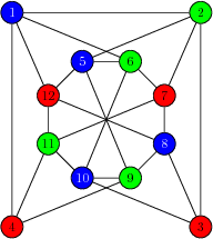
At this point it is sufficient to compute the Gröbner basis G of F = F_3 \cup F_{\mathcal{G}} to find out if a graph \mathcal{G} is 3–colorable, or not. After this theoretical introduction lets consider a graph \mathcal{G}(V, E) of figure The graph with 12 vertices and 23 edges, to see that the described scheme works in practice. We ask if the graph is 3–colorable. In this example we will first show how to answer this question SymPy and then we will compare this with three other symbolic manipulation systems on the market: Maxima, Axiom and Mathematica.

The graph \mathcal{G}(V, E)

The question, if \mathcal{G} is 3–colorable or not, is easy to answer by trial and error. We are, however, an interested in algorithmic solution to the problem, so lets first encode V and E of the graph \mathcal{G} using Python’s built–in data structures:

>>> V = range(1, 12+1)
>>> E = [(1,2),(2,3),(1,4),(1,6),(1,12),(2,5),(2,7),(3,8),
... (3,10),(4,11),(4,9),(5,6),(6,7),(7,8),(8,9),(9,10),
... (10,11),(11,12),(5,12),(5,9),(6,10),(7,11),(8,12)]

We encoded the set of vertices as a list of consecutive integers and the set of edges as a list of tuples of adjacent vertex indices. Next we will transform the graph into an algebraic form by mapping vertices to variables and tuples of indices into tuples of variables:

>>> Vx = [ Symbol('x' + str(i)) for i in V ]
>>> Ex = [ (Vx[i-1], Vx[j-1]) for i, j in E ]

As the last step of this construction we write equations for F_3 and F_{\mathcal{G}}:

>>> F3 = [ x**3 - 1 for x in Vx ]
>>> Fg = [ x**2 + x*y + y**2 for x, y in Ex ]

Everything is set following the theoretical introduction, so now we can compute the Gröbner basis of F_3 \cup F_{\mathcal{G}} with respect to lexicographic ordering of terms:

>>> G = groebner(F3 + Fg, Vx)

We know that if the constructed system of polynomial equations has a solution then G should be non–trivial, i.e. G \not= \emptyset, which can be easily verified in SymPy:

>>> G != [1]
True

The answer is that the graph \mathcal{G} is colorable with 3 colors. A sample coloring is shown in figure A sample –coloring of the graph . Suppose we add an edge between vertices i = 3 and j = 4. Is the new graph 3–colorable? To check this it is sufficient to construct F_{\mathcal{G'}} by extending F_{\mathcal{G}} with x_3^2 + x_3 x_4 + x_4^2 equation and recompute the Gröbner basis:

>>> x3, x4 = Vx[2], Vx[3]

>>> G = groebner(F3 + Fg + [x3**2 + x3*x4 + x4**2], Vx)

>>> G != [1]
False

We got a trivial Gröbner basis as the result, so the graph \mathcal{G'} isn’t 3–colorable. We could continue this discussion asking if \mathcal{G'} is 4–colorable or if the number of colors required to color the original graph could be lowered to 2 colors.

A sample 3–coloring of the graph \mathcal{G}(V, E)

Before we compare SymPy‘s syntax for computing Gröbner bases with other systems, let us clarify an issue arising around list indexing (e.g. why we write x3 = Vx[2]). SymPy is a library built on top of Python, so it utilizes Python’s built–in data structures and their indexing schemes. Python, as a general purpose programming language, uses well established zero–based indexing scheme, contrary to the natural way of indexing things, i.e. saying 1st, 2nd, 3rd etc. (to which we are accustomed in real life and mathematics). The zero–based indexing scheme dates back to the time of first programming languages, which were hardware oriented (e.g. assemblers) and an index was understood as an offset from a particular location in memory (the start of a container) to the requested item (for a more detailed discussion about this issue see [Dijkstra1982zero]). General purpose programming languages, even those interpreted like Python, coherently follow this scheme. For SymPy, this is a cost of building the system on top of a general purpose language. As we will see in the following examples, other symbolic manipulation systems, i.e. those which invent their own programming language, use natural indexing scheme. Currently a workaround to have one–based indexing in SymPy, is to append a dummy element in front of a list, e.g. to index Vx this way we could issue Vx = [None] + Vx and then x3 = Vx[3].

Vertex coloring using other systems¶

We showed so far how to solve classical vertex coloring problem with SymPy. Lets now compare SymPy‘s syntax and semantics of Gröbner bases functionality with three other mathematical software: Maxima, Axiom and Mathematica.

One feature that makes SymPy different from other mathematical systems is that SymPy utilizes a general purpose programming language for its core, modules and interaction with the user, whereas Maxima, Axiom and Mathematica invent their own special languages for implementing their mathematical libraries and for user interaction. This will require us to make some remarks also on the syntactic level.

Maxima, available at http://maxima.sourceforge.net, implements Gröbner bases in an extension library. Detailed documentation can be found in [MaximaGroebner]. We will reuse the same example and, as much as possible, the same computational approach. Maxima first requires us to load the Gröbner bases library. Note that we write grobner in this case. User should also remember about putting a semicolon at the end of every line. Next we define edges of the graph using a list of two element lists (there are no tuples in Maxima). Maxima uses very unusual syntax for variable assignment, utilizing colon for this purpose. In the next step we define the list of variables Vx and systems of polynomial equations F3 and Fg. Instead of list comprehensions we use makelist() function. One should note that Maxima uses ^ symbol for exponentiation, whereas Python uses this symbol for bitwise XOR operation. Finally we can compute the Gröbner basis using poly_reduced_grobner(). Maxima by default assumes lexicographic ordering of monomials. This information can be changed only by setting a global variable. As the last step we check if the computed basis is non–trivial, utilizing is() and notequal() functions. Lets see full source code for this example:

(i1) load(grobner);

(i2) E: [[1,2],[2,3],[1,4],[1,6],[1,12],[2,5],[2,7],[3,8],
[3,10],[4,11],[4,9],[5,6],[6,7],[7,8],[8,9],[9,10],[10,11],
[11,12],[5,12],[5,9],[6,10],[7,11],[8,12]];

(i3) Vx: makelist(concat("x", i), i, 1, 12);

(i4) F3: makelist(Vx[i]^3 - 1, i, 1, 12);
(i5) Fg: [];

(i6) for e in E do
        Fg: endcons(Vx[e[1]]^2 + Vx[e[1]]*Vx[e[2]] + Vx[e[2]]^2, Fg);

(i7) G: poly_reduced_grobner(append(F3, Fg), Vx);

(i8) is(notequal(G, [1]));
(o8) true

Axiom, available at http://axiom-developer.org, implements Gröbner bases toolkit in its core algebra library. The documentation on this matter, thought not very extensive, can be found in [Daly2003horizon]. Axiom uses a sophisticated autoloader of its library components, so explicit package loading in not necessary. As previously we start with the definition of the set of edges using a list of list. On should notice that, this time, the assignment operator is :=. Semicolons at the end of lines are not obligatory, however, useful for preventing printing of the results of computations. Next we define Vx and Ex in a way very similar to Python, as Axiom supports list comprehensions. The main difference is Axiom’s approach to indexing lists. Axiom does not use an object oriented language, as one might presume looking at the source code, and it doesn’t support properties. This give opportunity for reusing the dot operator for indexing purpose (notice also one–base indexes). Next definitions of F3 and Fg are almost equivalent to what we wrote using SymPy. Finally we compute the Gröbner basis using groebner() function. Notice the :: operator. It tells that the previously constructed polynomials should belong to the domain that is on its right hand side, i.e. distributed multivariate polynomial in symbols from Vx with coefficients over integers. At the end we check that the basis in non–trivial using ~= operator. Note that ~= is not a comparison operator by default, but returns an unequality, so we need to use coercion operator @ to tell ~= to end up with a Boolean result immediately. Here is the full source code for this example:

(1) -> E := [[1,2],[2,3],[1,4],[1,6],[1,12],[2,5],[2,7],
[3,8],[3,10],[4,11],[4,9],[5,6],[6,7],[7,8],[8,9],[9,10],
[10,11],[11,12],[5,12],[5,9],[6,10],[7,11],[8,12]];

(2) -> Vx := [ concat("x", i::String)::Symbol for i in 1..12 ];
(3) -> Ex := [ [Vx.(e.1), Vx.(e.2)] for e in E ];

(4) -> F3 := [ x**3 - 1 for x in Vx ];
(5) -> Fg := [ e.1**2 + e.1*e.2 + e.2**2 for e in Ex];

(6) -> G := groebner([ f::DMP(Vx, INT) for f in concat(F3, Fg) ]);

(7) -> (G ~= [1]) @ Boolean
   (7) true

Mathematica, available at http://www.wolfram.com/mathematica/, has extensive built–in support for Gröbner bases. Detailed documentation on this matter can be found in [MathematicaGroebner]. Mathematica has a very peculiar language for interaction with the user and its syntax, which was influence by the infix dialect of lisp (or m–lisp), is very different from other languages used in symbolic mathematics, so will skip detailed syntactic comparison and refer the reader to [Wolfram2003book].

In[1]:= Unprotect[E];
In[2]:= E := {{1,2},{2,3},{1,4},{1,6},{1,12},{2,5},{2,7},
{3,8},{3,10},{4,11},{4,9},{5,6},{6,7},{7,8},{8,9},{9,10},
{10,11},{11,12},{5,12},{5,9},{6,10},{7,11},{8,12}}

In[3]:= Vx := Table[Symbol["x" <> ToString[i]], {i,1,12}]
In[4]:= h[{i_, j_}] := Vx[[i]]^2 + Vx[[i]] Vx[[j]] + Vx[[j]]^2

In[5]:= F3 := Map[(#^3-1)&, Vx]
In[6]:= Fg := Map[h, E]

In[7]:= G := GroebnerBasis[Join[F3, Fg], Vx]

In[8]:= G != {1}
Out[8]= True

We showed how to perform classical vertex coloring of a graph based on the Gröbner bases method using SymPy and three other mathematical systems. It is interesting to compare the times that were needed to compute the Gröbner basis G by each of those systems. Timings (average of multiple runs) were collected in figure Average timing for computing Gröbner basis of graph . This simple study shows that both SymPy and Maxima are significantly slower than Axiom and Mathematica. This happens, because the implementation of Gröbner bases in both systems is done in an interpreted language (Python and Maxima language, respectively). Possibly they also implement less(–powerful) criteria for eliminating useless critical pairs.

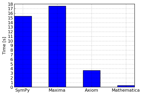
Average timing for computing Gröbner basis of graph \mathcal{G}(V, E)

>>> zeta = exp(2*pi*I/3).expand(complex=True)

>>> zeta
    ___
I⋅╲╱ 3
─────── - 1/2
   2

>>> factor(x**3 - 1, extension=zeta)
        ⎛        ___      ⎞ ⎛        ___      ⎞
        ⎜    I⋅╲╱ 3       ⎟ ⎜    I⋅╲╱ 3       ⎟
(x - 1)⋅⎜x + ─────── + 1/2⎟⋅⎜x - ─────── + 1/2⎟
        ⎝       2         ⎠ ⎝       2         ⎠

>>> [ solve(arg)[0] for arg in _.args ]
⎡         ___            ___      ⎤
⎢     I⋅╲╱ 3         I⋅╲╱ 3       ⎥
⎢1, - ─────── - 1/2, ─────── - 1/2⎥
⎣        2              2         ⎦

>>> var('red,green,blue')
(red, green, blue)

>>> colors = zip(__, _)

>>> colors
⎡          ⎛      ___             ⎞  ⎛    ___            ⎞⎤
⎢          ⎜  I⋅╲╱ 3              ⎟  ⎜I⋅╲╱ 3             ⎟⎥
⎢(1, red), ⎜- ─────── - 1/2, green⎟, ⎜─────── - 1/2, blue⎟⎥
⎣          ⎝     2                ⎠  ⎝   2               ⎠⎦

>>> key = lambda f: (degree(f), len(f.args))
>>> groups = split(G, key, reverse=True)

>>> len(groups)
4

>>> groups[0]
⎡   3    ⎤
⎣x₁₂  - 1⎦

>>> groups[1]
⎡   2                2⎤
⎣x₁₁  + x₁₁⋅x₁₂ + x₁₂ ⎦

>>> groups[2]
[x₁ + x₁₁ + x₁₂, x₁₁ + x₁₂ + x₅, x₁₁ + x₁₂ + x₈, x₁₀ + x₁₁ + x₁₂]

>>> groups[3]
[-x₁₁ + x₂, -x₁₂ + x₃, -x₁₂ + x₄, -x₁₁ + x₆, -x₁₂ + x₇, -x₁₁ + x₉]

>>> colorings = solve(G, Vx)

>>> len(colorings)
6

>>> for coloring in colorings:
...     print [ elt.expand(complex=True).subs(colors) for elt in coloring ]
...
...
[blue, green, red, red, blue, green, red, blue, green, blue, green, red]
[green, blue, red, red, green, blue, red, green, blue, green, blue, red]
[green, red, blue, blue, green, red, blue, green, red, green, red, blue]
[red, green, blue, blue, red, green, blue, red, green, red, green, blue]
[blue, red, green, green, blue, red, green, blue, red, blue, red, green]
[red, blue, green, green, red, blue, green, red, blue, red, blue, green]

Algebraic geometry¶

Geometry is one of the primary subjects taught during elementary mathematics classes and using SymPy for studying theorems of Euclidean geometry seems a very promising idea. For example, lets consider a rhombus (in a fixed coordinate system). We would like to prove a theorem that diagonals of a rhombus are mutually perpendicular. We are of course interested in a purely algorithmic approach to solve this problem. To prove this theorem we will use the machinery of Gröbner bases.

Following [Winkler1990geometry], lets consider a geometric entity which properties can be translated into a system of m polynomials, say \mathcal{H} = \{f_1, \ldots, f_m\}. We will call \mathcal{H} a hypothesis. Given a theorem concerning this geometric entity, the algebraic formulation is as follows:

where g is the conclusion of the theorem and f_1, \ldots f_m and g are polynomials in \K[x_1, \ldots, x_n, y_1, \ldots, y_n]. It follows from the Gröbner bases theory that the above statement is true when g belongs to the ideal generated by \mathcal{H}. To check this, i.e. to prove the theorem, it is sufficient to compute Gröbner basis of \mathcal{H} and reduce g with respect to this basis. If the theorem is true then the remainder from the reduction will vanish. In this example, for the sake of simplicity, we assume that the geometric entity is non–degenerate, i.e. it does not collapse into a line or a point. Anyway, the Gröbner basis approach allows to prove theorems in algebraic geometry in full generality and derive automatically non–degeneracy conditions.

A rhombus in a fixed coordinate system

Lets consider the rhombus of figure A rhombus in a fixed coordinate system. This geometric entity consists of four points A, B, C and D. To setup a fixed coordinate system, without loss of generality, we can assume that A = (0, 0), B = (x_B, 0), C = (x_C, y_C) and D = (x_D, y_D). This is possible by taking rotational invariance of the geometric entity. We will prove that the diagonals of this rhombus, i.e. AD and BC are mutually perpendicular. We have the following conditions describing ABCD:

1. Line AD is parallel to BC, i.e. AD \parallel BC.
2. Sides of ABCD are of the equal length, i.e. AB = BC.
3. The rhombus is non–degenerate, i.e. is not a line or a point.

Our conclusion is that AC \bot BD. To prove this theorem, first we need to transform the above conditions and the conclusion into a set of polynomials. How we can achieve this? Lets focus on the first condition. In general, we are given two lines A_1A_2 and B_1B_2. To express the relation between those two lines, i.e. that A_1A_2 is parallel B_1B_2, we can relate slopes of those lines:

Clearing denominators in the above expression and putting all terms on the left hand side of the equation, we derive a general polynomial describing the first condition. This can be literally translated into Python:

def parallel(A1, A2, B1, B2):
    """Line [A1, A2] is parallel to line [B1, B2]. """
    return (A2.y - A1.y)*(B2.x - B1.x) - (B2.y - B1.y)*(A2.x - A1.x)

assuming that A1, A2, B1 and B2 are instances of Point class. In the case of our rhombus, we will take advantage of the fixed coordinate system and simplify the resulting polynomials as much as possible. The same approach can be used to derive polynomial representation for other conditions and the conclusion. To construct \mathcal{H} and g we will use the following functions:

def distance(A1, A2):
    """The squared distance between points A1 and A2. """
    return (A2.x - A1.x)**2 + (A2.y - A1.y)**2

def equal(A1, A2, B1, B2):
    """Lines [A1, A2] and [B1, B2] are of the same width. """
    return distance(A1, A2) - distance(B1, B2)

def perpendicular(A1, A2, B1, B2):
    """Line [A1, A2] is perpendicular to line [B1, B2]. """
    return (A2.x - A1.x)*(B2.x - B1.x) + (A2.y - A1.y)*(B2.y - B1.y)

The non–degeneracy statement requires a few words of comment. Many theorems in geometry are true only in the non–degenerative case and false or undefined otherwise. In our approach to theorem proving in algebraic geometry, we must supply sufficient non–degeneracy conditions manually. In the case of our rhombus this is x_B > 0 and y_C > 0 (we don’t need to take x_C into account because AB = BC). At first, this seems to be a show stopper, as Gröbner bases don’t support inequalities. However, we can use Rabinovich trick and transform those inequalities into a single polynomial condition by introducing an additional variable, say a, about which we will assume that is positive. This gives us a non–degeneracy condition x_B y_C - a.

With all this knowledge we are ready to prove the main theorem. First, lets declare variables:

>>> var('x_B, x_C, y_C, x_D, a')
(x_B, x_C, y_C, x_D, a)

>>> vars = _[:-1]

We had to declare the additional variable a, but we don’t consider it a variable of our problem. This will lead to a new case in SymPy‘s implementation of Gröbner bases, because we will be computing not over rationals, as we did in all previous examples, but the computations will be done over the field of univariate rational functions. Lets now define the four points A, B, C and D:

>>> A = Point(0, 0)
>>> B = Point(x_B, 0)
>>> C = Point(x_C, y_C)
>>> D = Point(x_D, y_C)

Using the previously defined functions we can define the hypothesis:

>>> h1 = parallel(A, D, B, C)
>>> h2 = equal(A, B, B, C)
>>> h3 = x_B*y_C - a

and compute its Gröbner basis:

>>> G = groebner([h1, h2, h3], vars, order='grlex')

Two things need a comment here. Previously we specified variables in groebner(), when we were concerned about the order of variables. This was necessary when the task was to eliminate particular variables, before proceeding to the other steps of an algorithm. However, in this case we are rather concerned about not letting the variable a to be considered as a significant variable in the problem, because we treat a as a parameter. The other thing is that we can compute the Gröbner basis with respect to any admissible ordering of monomials. We chose the standard total degree scheme, over the default lexicographic ordering, because leads to shorter computation times.

Lets now verify the theorem:

>>> reduced(perpendicular(A, C, B, D), G, vars, order='grlex')[1]
0

This proves that AC \bot BD. Although, the theorem we described and proved was a simple one, one can handle much more complicated problems as well. One should refer to Winkler’s paper for more interesting examples, especially concerning issues with degenerate cases.

Other applications¶

So far several detailed examples of practical applications of the Gröbner bases method were presented, which explained most interesting features of Gröbner bases and their use patterns in SymPy. Following the list from the beginning of this section, there are, however, many more applications. We will give reference to several of them in this part.

Besides the obvious application of solving systems of polynomial equations and the less obvious for computing LCMs and GCDs of multivariate polynomials, the Gröbner basis method is also used in SymPy for computing minimal polynomials of algebraic numbers, primitive elements of algebraic fields and isomorphisms between algebraic fields (for a detailed theoretical discussion see [Adams1994intro] and algorithms refer to [Cohen1993course]). For all those tasks there are much more efficient algorithms implemented in SymPy. However, Gröbner bases remain the fallback tool if any of the fast algorithms isn’t suitable for a particular job. For example, minimal polynomials can be relatively easily computed using PSLQ algorithm (see pslq() function in mpmath library) but only in the case of real algebraic numbers. In the more general case of complex algebraic numbers the Gröbner bases method is the only choice.

Gröbner bases can be also directly applicable in symbolic manipulation systems for computing factorizations of multivariate polynomials [Gianni1985groebner] or evaluating symbolic summations and integrals [Chyzak1998groebner].