Not only symbolics: numerical computing

Symbolic mathematics can’t exist without numerical methods. Most “symbolic” modules in SymPy take at least some advantage of numerical computing. SymPy uses the mpmath library for this purpose.

Let’s start from something simple and find numerical approximation to \(\pi\). Normally SymPy represents \(\pi\) as a symbolic entity:

>>> pi
π
>>> type(_)
<class 'sympy.core.numbers.Pi'>

To obtain numerical approximation of \(\pi\) we can use either the evalf() method or N(), which is a simple wrapper over the former method:

>>> pi.evalf()
3.14159265358979

The default precision is 15 digits. We can change this using the n parameter:

>>> pi.evalf(n=30)
3.14159265358979323846264338328

The mpmath library implements arbitrary precision floating point arithmetics (limited only by available memory), so we can set n to a very big value, e.g. one million:

>>> million_digits = pi.evalf(n=1000000)
>>> str(million_digits)[-1]
5

evalf() can handle much more complex expressions than \(\pi\), for example:

>>> exp(sin(1) + E**pi - I)
           π
 sin(1) + ℯ  - ⅈ
ℯ

>>> _.evalf()
14059120207.1707 - 21895782412.4995⋅ⅈ

or:

>>> zeta(S(14)/17)
 ⎛14⎞
ζ⎜──⎟
 ⎝17⎠

>>> zeta(S(14)/17).evalf()
-5.10244976858838

Note that in SymPy, exp(1) is denoted by capital :exp:E

>>> E.evalf()
2.71828182845905

Symbolic entities are ignored:

>>> pi*x
π⋅x
>>> _.evalf()
3.14159265358979⋅x

Built-in functions float() and complex() take advantage of evalf():

>>> float(pi)
3.14159265359
>>> type(_)
<type 'float'>

>>> float(pi*I)
Traceback (most recent call last):
...
ValueError: Symbolic value, can't compute

>>> complex(pi*I)
3.14159265359j
>>> type(_)
<type 'complex'>

The base type for computing with floating point numbers in SymPy is Float. It allows for several flavors of initialization and keeps track of precision:

>>> 2.0
2.0
>>> type(_)
<type 'float'>

>>> Float(2.0)
2.00000000000000
>>> type(_)
<class 'sympy.core.numbers.Float'>

>>> sympify(2.0)
2.00000000000000
>>> type(_)
<class 'sympy.core.numbers.Float'>

>>> Float("3.14")
3.14000000000000
>>> Float("3.14e-400")
3.14000000000000e-400

Notice that the last value is out of range for float:

>>> 3.14e-400
0.0

We expected a very small value but not zero. This raises an important issue, because if we try to construct a Float this way, we will still get zero:

>>> Float(3.14e-400)
0

The only way to fix this is to pass a string argument to Float.

When symbolic mathematics matter?

Consider a univariate function:

\[f(x) = x^{(1 - \log(\log(\log(\log(\frac{1}{x})))))}\]

We would like to compute:

\[\lim_{x \to 0^{+}} f(x)\]

Let’s define the function \(f\) in SymPy:

>>> f = x**(1 - log(log(log(log(1/x)))))
>>> f
      ⎛   ⎛   ⎛   ⎛1⎞⎞⎞⎞
 - log⎜log⎜log⎜log⎜─⎟⎟⎟⎟ + 1
      ⎝   ⎝   ⎝   ⎝x⎠⎠⎠⎠
x

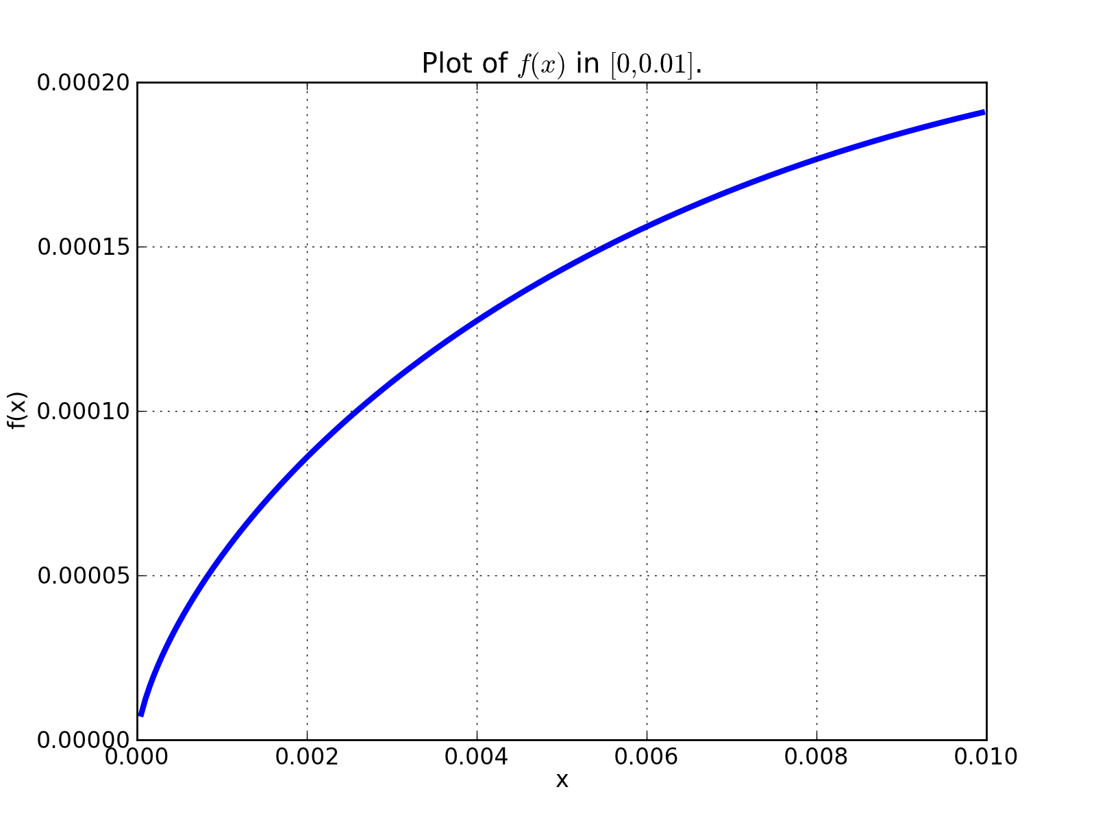
A very straight forward approach is to “see” how \(f\) behaves on the right hand side of zero. We can try to read the solution from the graph of \(f\):

import matplotlib.pyplot as plt
from sympy.mpmath import plot, log

fig = plt.figure()
axes = fig.add_subplot(111)
axes.set_title(r"Plot of $f(x)$ in $[0, 0.01]$.")

f = lambda x: x**(1 - log(log(log(log(1/x)))))
plot(f, xlim=[0, 0.01], axes=axes)

(Source code, png, hires.png, pdf)

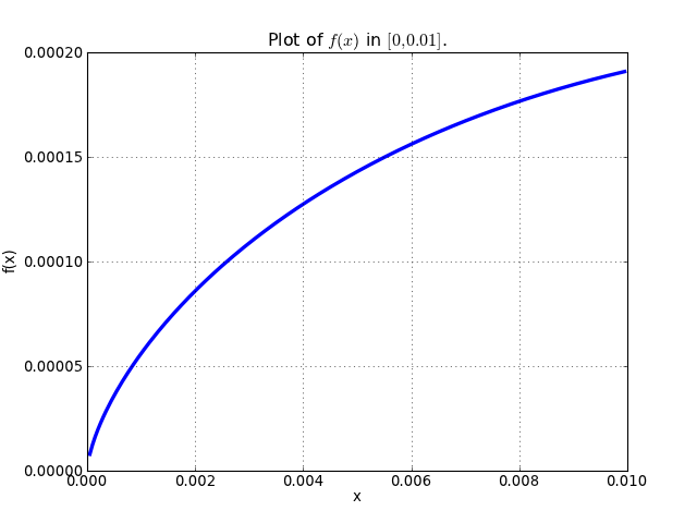
This gives us first hint that the limit might be zero. Of course reading a graph of a function isn’t a very precise method for computing limits. Instead of analyzing the graph of \(f\), we can improve this approach a little by evaluating \(f(x)\) for sufficiently small arguments.

Let’s start with arguments of the form \(x = 10^{-k}\):

>>> f.subs(x, 10**-1).evalf()
0.00114216521536353 + 0.00159920801047526⋅ⅈ
>>> f.subs(x, 10**-2).evalf()
0.000191087007486009
>>> f.subs(x, 10**-3).evalf()
5.60274947776528e-5
>>> f.subs(x, 10**-4).evalf()
1.24646630615307e-5
>>> f.subs(x, 10**-5).evalf()
2.73214471781554e-6
>>> f.subs(x, 10**-6).evalf()
6.14631623897124e-7
>>> f.subs(x, 10**-7).evalf()
1.42980539541700e-7
>>> f.subs(x, 10**-8).evalf()
3.43858142726788e-8

We obtained a decreasing sequence values which suggests that the limit is zero. Let’s now try points of the form \(x = 10^{-10^k}\):

>>> f.subs(x, 10**-10**1).evalf()
2.17686941815359e-9
>>> f.subs(x, 10**-10**2).evalf()
4.87036575966825e-48
>>> f.subs(x, 10**-10**3).evalf()
+inf

For \(x = 10^{-10^3}\) we got a very peculiar value. This happened because:

>>> 10**-10**3
0.0

and the reason for this is that we used Python’s floating point values. Instead we can use either exact numbers or SymPy’s floating point numbers:

>>> Integer(10)**-10**3 != 0
True
>>> Float(10.0)**-10**3 != 0
True

Let’s continue with SymPy’s floating point numbers:

>>> f.subs(x, Float(10.0)**-10**1).evalf()
2.17686941815359e-9
>>> f.subs(x, Float(10.0)**-10**2).evalf()
4.87036575966825e-48
>>> f.subs(x, Float(10.0)**-10**3).evalf()
1.56972853078736e-284
>>> f.subs(x, Float(10.0)**-10**4).evalf()
3.42160969045530e-1641
>>> f.subs(x, Float(10.0)**-10**5).evalf()
1.06692865269193e-7836
>>> f.subs(x, Float(10.0)**-10**6).evalf()
4.40959214078817e-12540
>>> f.subs(x, Float(10.0)**-10**7).evalf()
1.11148303902275e+404157
>>> f.subs(x, Float(10.0)**-10**8).evalf()
8.63427256445142e+8443082

This time the sequence of values is rapidly decreasing, but only until a sufficiently small numer where \(f\) has an inflexion point. After that, values of \(f\) increase very rapidly, which may suggest that the actual limit is +\inf. It seems that our initial guess is wrong. However, for now we still can’t draw any conclusions about behavior of \(f\), because if we take even smaller numbers we may reach other points of inflection.

The mpmath library implements a function for computing numerical limits of function, we can try to take advantage of this:

>>> from sympy.mpmath import limit as nlimit
>>> F = lambdify(x, f, modules='mpmath')

>>> nlimit(F, 0)
(2.23372778188847e-5 + 2.28936592344331e-8j)

This once again suggests that the limit is zero. Let’s use an exponential distribution of points in nlimit():

>>> nlimit(F, 0, exp=True)
(3.43571317799366e-20 + 4.71360839667667e-23j)

This didn’t help much. Still zero. The only solution to this problem is to use analytic methods. For this we will use limit():

>>> limit(f, x, 0)
∞

which shows us that our initial guess was completely wrong. This nicely shows that solving ill conditioned problems may require assistance of symbolic mathematics system. More about this can be found in Dominic Gruntz’s PhD tesis (http://www.cybertester.com/data/gruntz.pdf), where this problem is explained in detail and an algorithm shown, which can solve this problem and which is implemented in SymPy.

Tasks

1. Compute first 55 digits of numerical approximation of \(f(\pi)\).

   (solution)

2. Read this webcomic. What is the first digit of \(e\) to contain \(999999\)? What is the first digit of \(\pi\) to contain \(789\)?

   (solution)

3. In addition to the above example, Gruntz gives another example of ill conditioned function in his thesis to show why symbolic computation of limits can be preferred to numerical computation:

   \[\lim_{x \to \infty}{\left(\operatorname{erf}\left(x - {e^{-e^{x}}}\right) - \operatorname{erf}\left(x\right)\right) e^{e^{x}}} e^{x^{2}}\]

   (in SymPy, (erf(x - exp(-exp(x))) - erf(x))*exp(exp(x))*exp(x**2)). Compute the above limit in SymPy using methods similar to the ones presented in this section. What are the drawbacks of computing this limit numerically? What is the limit, exactly?

   (solution)