Notes on the internal implementation¶

Motivation¶

Why we need exactly four levels in polynomials manipulation module? Suppose we need to compute a factorization of polynomial x^{10} - 1. There are four levels, so we can perform the same computation in four different ways:

>>> f3 = x**10 - 1
>>> %timeit factor_list(f3)
100 loops, best of 3: 5.57 ms per loop

>>> f2 = Poly(x**10 - 1, x, domain='ZZ')
>>> %timeit f2.factor_list()
100 loops, best of 3: 2.15 ms per loop

>>> f1 = DMP([mpz(1), mpz(0), mpz(0), mpz(0), mpz(0),
... mpz(0), mpz(0), mpz(0), mpz(0), mpz(0), mpz(-1)], ZZ)
>>> %timeit f1.factor_list()
100 loops, best of 3: 1.90 ms per loop

>>> f0 = [mpz(1), mpz(0), mpz(0), mpz(0), mpz(0),
... mpz(0), mpz(0), mpz(0), mpz(0), mpz(0), mpz(-1)]
>>> %timeit dup_factor_list(f0, ZZ)
100 loops, best of 3: 1.88 ms per loop

We factored polynomial x^{10} - 1 starting with the highest level and ending on the lowest level. On L3 we used an expression to construct the polynomial and we did not have to pay any attention to the details, which were figured out automatically by factor_list() function. On L2 we created a polynomial explicitly by providing a generator and coefficient domain. This time we used factor_list() method of Poly. This computation took less than half of time that was needed to compute the same thing on L3. Next we performed the same computation on L1 level, the first internal level of the module, constructing the polynomial by providing an explicit polynomial representation (dense in this case) and we gained a 10% speedup. Finally we computed the factorization on the lowest level, gaining tiny speed improvement.

We can see that, depending on the level on which we performed the computation, we had to pay increasingly more attention to the technical details, but we gained speed improvement thanks to this. The improvement might not seem very encouraging, especially when we compare levels L2, L1 and L0. However, we have to keep in mind that those milli– or microseconds that we save with each computation, have to be multiplied by the number of all computations we do, and from this perspective we do not save only fractions of seconds but we save seconds or even minutes or hours of computation time.

The zeroth level: L0¶

This is the lowest level of polynomials manipulation functionality, which is used only for internal purpose of the module. Most algorithms that the module implements, especially those which are most commonly used as parts of other algorithms or are most computationally demanding, are implemented on this level. This includes algorithms for polynomial arithmetics, GCD and LCM computation, square–free decomposition, polynomial factorization, root isolation, Gröbner bases and others.

To reduce the overhead of Python to minimum, the zeroth level is implemented in purely procedural style: it consists only of functions and all data is passed explicitly via arguments to functions. On this level we do not take advantage of any runtime magic like context managers, everything is done explicitly. Besides being fast, this has also the benefit that the code is very verbose and thus easily understandable, which is not often the case in object–oriented programming. It might seem a bit awkward, after so many years of declining of procedural programming, to use this old fashioned style, but currently it seems the right choice. Although, in the opinion of the author, procedural code is easy to understand, it is not that easy to write, especially for newcomers, because of very high level of verboseness of such code. However, this is the trade–off we have to make, to make SymPy both usable and reasonably fast.

Functions on this level are spread over several source files in sympy/polys and are split into groups, depending on which polynomial representation they belong to and what kind of ground domain can be used with them. Currently there are four major groups, which can be distinguished by their special prefixes:

• gf_ — dense univariate polynomials over finite (Galois) fields
• dup_ — dense univariate polynomials over arbitrary domains
• dmp_ — dense multivariate polynomials over arbitrary domains
• sdp_ — sparse distributed polynomials over arbitrary domains

There are additional minor suffixes, which can be added to the major prefixes. They are used to tell the difference between the same function, e.g. for computing the greatest common divisor, for various ground domains. The typically used suffixes are zz_, qq_, rr_ and ff_, which stand for the ring of integers, the rational field, a ring and a field, respectively. Note that those suffixes are not combined with the gf_ prefix, which already limits the possible ground domains to a single one. Usually, if a function comes with a suffix, then it will be defined for both, either zz_ and qq_, or rr_ and ff_ suffixes. There will be also a function without any suffix, which will dispatch the flow to an appropriate function for a specialized ground domain, depending on the analysis of the ground domain argument to this function. This separation is necessary, because it often happens that functions for computing a particular thing over different ground domains, have very different semantics and internal structure. A good examples are functions for computing GCDs and factorizations of polynomials. One should also note that even if there is a separation between different ground domains, it is still possible (and it often happens) that a function for a more general domain will transform the problem and run an algorithm for a smaller domain, to take advantage of more efficient algorithms.

Although we listed four groups of types of functions, there are really only three true groups, because dup_ and dmp_ depend on each other, forming a larger group. This is because dmp_ functions use dup_ function to terminate recurrence, as dmp_ implement dense recursive representation.

Suppose we want to implement a function for computing Taylor shifts. Given a univariate polynomial f in \K[x], where \K is an arbitrary domain, and a value a \in \K, we call a Taylor shift an evaluation of f(x + a). For details of the algorithm refer to [Nijenhuis1978combinatorial]. To focus our attention, we will show a sample implementation Taylor shift algorithm only for dense polynomial representation. The implementation may be as follows:

@cythonized('n,i,j')
def dup_taylor(f, a, K):
    """Evaluate efficiently Taylor shift ``f(x + a)`` in ``K[x]``. """
    f, n = list(f), dup_degree(f)

    for i in xrange(n, 0, -1):
        for j in xrange(0, i):
            f[j+1] += a*f[j]

    return f

We defined a function called dup_taylor which takes three arguments: f, a and K. We followed here the standard convention of L0 level, where dup_ prefix tells us that the function uses dense polynomial representation and allows only univariate polynomials. In the arguments list, the first argument is an input polynomial, the second is evaluation point a and the last one is the coefficient domain. If a function requires two polynomials as input, e.g. multiplication function, then the first two arguments are polynomials and other arguments come next. However, the domain is always the last one (not counting optional or keyword–only arguments, which are rarely used on this level).

This was for dense univariate polynomials. The convention for other groups of functions varies a little bit. In the case of dense multivariate polynomials we add an additional argument u, which always goes before the ground domain, and stands for the number of variables of the input polynomial minus one. Thus we get zero for univariate polynomials, which is convenient, because in the univariate case, we can efficiently check that the polynomial is really univariate and fallback to the equivalent univariate function to terminate recurrence. In the case of sparse distributed polynomials we add another argument O, besides u, which goes between u and K, and stands for a function that defines an ordering relation between monomials (more about monomial orderings can be found in section Admissible orderings of monomials).

A very special case is the group of gf_ functions, which are used for computations with polynomials over finite fields. The convention in this case is that the domain K is some domain representing the ring of integers, not finite fields. We add an additional argument p, which goes before K and stands for the size of the finite field (modulus). This, somehow awkward convention, has purely historical background, because when L0 level was invented there were no ground domains in SymPy, so the argument p was the way to pass knowledge about the finite field, in which computations are done, to gf_ function. When ground domains were added to SymPy, then it was too costly at that time to remove argument p and use finite field domains instead of integer ring domains. It was also uncertain if such move would not add too much overhead and slowdown gf_ functions. A study is needed to show if there is any advantage at all of having separate group of functions for the special case of finite fields. Possibly in near future gf_ functions will be merged with dup_ functions, and gf_ will be transformed to a suffix, because still finite fields are special because specialized algorithms are needed for performing computations over this domain.

The first level: L1¶

This is the second level in polynomials manipulation module and the last level used for internal purpose. It is implemented in object–oriented style and wraps up functionality of the lowest level into four classes: GFP, DUP, DMP and SDP. Each class has methods which reflect functions of L0 level, but with prefixes stripped. Also method call convention changes, because ground domain and other properties are included in instances of L1 classes and provided only on class initialization. This makes usage of functionality exposed by this level more efficient, because the code is not that verbose as on the lowest level. L1 also implements several other classes which provide more general computational tools, e.g. DMF for dense multivariate fractions and ANP for a representation of algebraic numbers.

Classes of L1 level add tiny overhead over L0 functions, because L1 allows for unification polynomials if they have different ground domains and there is additional constant time needed to construct instances of L1 classes. In general in SymPy we allow only immutable classes, so instantiation overhead is added with every computation.

The main task for L1 level, besides wrapping up functionality of the lowest level, is to provide types (classes) which can be used in composite ground domains, i.e. polynomial, rational function and algebraic domains. We could use for this purpose tools of levels L2 and L3, but overhead associated with them would be too significant and thus computations with composite ground domains would be very inefficient. This way levels L0 and L1 define a self contained computational model for polynomials, which is later wrapped in much more user friendly levels L2 and L3, which we will describe next.

The second level: L2¶

This is the first level in polynomials manipulation module that is oriented towards the end user. We implement only one class in L2, Poly, which wraps up by composition GFP, DUP, DMP and SDP classes of L1, which we call, in this setup, polynomial representations. The class of L2 implements the union of all methods that are available in L1 classes. If certain operation is not supported by an underlying representation, OperationNotSupported exception is raised. Otherwise, during a method call of Poly high–level input arguments are converted to lower–level representations and passed to L1 level. When L1 finishes, output is converted back to high–level representations.

Poly implements expression parser, which allows to construct polynomials not only from raw polynomial representations, e.g. a list of coefficients, but it can also parse SymPy‘s expressions and translate them to a desired polynomial representation. It is also possible to automatically derive as much information as possible about an expression, without forcing the user to provide additional information manually. For example Poly can figure out the generators and the domain of expression on its own. This is very useful functionality, especially in interactive sessions, because it allows to significantly cut on typing.

The third level: L3¶

To make the functionality, provided by the module, more accessible by the user, most methods of Poly are exposed to the top–level via global functions of L3 level. Those functions allow to use procedural interface to the module, making it appealing to users, who have already some experience in other symbolic mathematics software. There are also some additional functions, which wrap more general functions and allow to take advantage of their behaviour in some specific way. For example, there is a method of L2 and a function of L3, factor_list(), which returns a list of irreducible factors of a polynomial. L3 implements an additional function factor() which uses factor_list() to compute factorization of a polynomial, but instead of returning a list, it returns an expression in factored (multiplicative) form.

The Poly and all functions exposed by L3 level are called the public API of polynomials manipulation module. The public API is the outcome of from sympy.polys import * statement. It is, however, not an issue to import other functions and classes from the module. The user should be aware that only the public API implements user–friendly interface and using lower–level tools might be a pain, for example in interactive sessions. To cut on redundancy, the reader should refer to section Motivation to see example of the same computation done on different levels of polynomials manipulation module. During the typical usage of SymPy, only the public API, i.e. levels L2 and L3, are be necessary.

Multiple–levels in practice¶

Suppose we are given a univariate polynomial with integer coefficients:

We ask what is the value of f at some specific point, say 15. We can achieve this by substituting 15 for x using subs() method of Basic (the root class in SymPy). This might not seem to be the optimal solution for the problem, because subs() does not take advantage of the structure of an input expression, just applies blindly pattern matching and SymPy’s built–in evaluation rules. This is, however, the first approach we can come out with, so lets try it:

>>> f = 3*x**17 + 3*x**5 - 20*x**2 + x + 17

>>> f.subs(x, 15)
295578376007082351782

As the solution we obtained a very large number which is greater than 2^{64}, i.e. can’t fit into CPU registers of modern machines. This is not an issue, because SymPy reuses Python’s arbitrary length integers, which are only bounded by the size of available memory. The size of the computed value might, however, raise a question concerning the speed of evaluation. As we said, subs() is a very naive function. Lets see how fast it can be:

>>> %timeit f.subs(x, 15);
1000 loops, best of 3: 992 us per loop

It takes subs() about one millisecond to compute f(15). This seems not that bad at all, especially in an interactive session, because one millisecond is not measurable about of time for the user. Lets check if we get the same behaviour for much larger evaluation points:

>>> %timeit f.subs(x, 15**20);
1000 loops, best of 3: 1.03 ms per loop

We chose a relatively large number 15^{20} for this test and obtained increase in evaluation time by a very small fraction. This is still fine in an interactive session, but would it be acceptable if subs() was used as a component of another algorithm, which requires several thousandths of evaluations? Lets consider a more demanding example. We now use random_poly() function to generate a polynomial of large degree to see how subs() scales when the size of the problem increases:

>>> g = random_poly(x, 1000, -10, 10)

>>> %time g.subs(x, 15);
CPU times: user 7.03 s, sys: 0.00 s, total: 7.03 s
Wall time: 7.20 s

This time the results are not encouraging at all. We got 7 seconds of evaluation time, for a polynomial of the degree 1000 with integer coefficients bounded by -10 and 10. This is not acceptable even in an interactive session. It gets even worse if we do the computation using the larger evaluation point:

>>> %time g.subs(x, 15**20);
CPU times: user 9.88 s, sys: 0.04 s, total: 9.91 s
Wall time: 10.29 s

Can we do better than this? To improve this timing we need to take advantage of the structure of the input expressions, i.e. recognize that both f and g are univariate polynomial with a very simple kind of coefficients — integers. This knowledge is very important, because we can pick up an optimized algorithm for this particular domain of computation. A well known algorithm for evaluating univariate polynomial is Horner’s scheme, which is implemented in eval() method of Poly class. Lets rewrite f and g as polynomials and redo the timings:

>>> F = Poly(f)
>>> G = Poly(g)

>>> %timeit F.eval(15);
10000 loops, best of 3: 34.3 us per loop

>>> %timeit F.eval(15**20);
10000 loops, best of 3: 43.1 us per loop

>>> %timeit G.eval(15);
1000 loops, best of 3: 1.02 ms per loop

>>> %timeit G.eval(15**20);
100 loops, best of 3: 16.4 ms per loop

We used Poly to obtain polynomials form of f and g, arriving with polynomials F and G respectively. We can clearly see, especially in the case of the large degree polynomial, that eval() introduced a significant improvement in execution times. This is not an accident, because eval() uses a dedicated algorithm for the task and, what is currently not visible, takes advantage of gmpy library, a very efficient library for doing integer arithmetics. This may be considered as a cheat, so lets force Poly to compute with SymPy’s built–in integer type:

>>> from sympy.polys.algebratools import ZZ_sympy

>>> FF = Poly(f, domain=ZZ_sympy())
>>> GG = Poly(g, domain=ZZ_sympy())

>>> %timeit FF.eval(15);
1000 loops, best of 3: 226 us per loop

>>> %timeit FF.eval(15**20);
1000 loops, best of 3: 283 us per loop

>>> %timeit GG.eval(15);
100 loops, best of 3: 15.7 ms per loop

>>> %timeit GG.eval(15**20);
10 loops, best of 3: 123 ms per loop

We obtained a visible slowdown, but we are still much faster that when using subs(). A careful reader would argue that those timings are cheating once again, because we did not take in to account the construction times of Poly class instances. Lets check if this is significant:

>>> %timeit Poly(f);
100 loops, best of 3: 6.54 ms per loop

>>> %timeit Poly(g);
1 loops, best of 3: 1.79 s per loop

Indeed, construction of polynomials in this setup seems a very time consuming procedure. In the case of the expression f we do even worse that when using subs() alone. In the later case we are still better, but the difference is not that impressive anymore. Although this timing might look fine to the reader, it is a complete non–sense in this comparison. This is because Poly class constructor expands the input expression by default and this step takes majory of initialization time:

>>> %timeit G = Poly(f, expand=False)
1000 loops, best of 3: 209 us per loop

>>> %timeit G = Poly(g, expand=False)
10 loops, best of 3: 20.2 ms per loop

We know that f and g are already in the expanded form, so we can safely set expand option to False and completely skip the expansion step. This gives us a significant speedup, when compared to the previous timing. The reader should not get distracted by this issue, because the reason for which expand(), a function which is used for expanding expressions, is so slow, is because of its bulky implementation, which will change in near future. Thus, there will be no need to bother with expand option.

Why eval() function of Poly is so fast? One reason we already know, it uses an optimized algorithm for its task and it takes advantage over very fast integers. However, this is only a part of the story. The other is its implementation. eval() is implemented on the lowest level — L0. There are no overheads that are associated with computations with symbolic expressions, thus we obtain very short execution times.

Dense polynomial representation¶

It is worthwhile to define dense polynomial representation only for univariate polynomials. In this case the representation of a polynomial of degree n is a list with n+1 elements:

Those elements are all coefficients, including zeros, of a polynomial, in order from the term with the highest degree (\mbox{coeff}_n \cdot x^n) to the constant term (\mbox{coeff}_0). Thus, if we ask for the leading coefficients (or monomial, or term), then this is always the first element of dense univariate polynomial representation. If a polynomial is the zero polynomial, i.e. it has negative degree, then the representation is simply the empty list. This is useful attitude, because we can check very efficiently if we obtained the zero polynomial during computations. Dense univariate representation is a very important tool in applications were all or most terms of polynomials are non–zero. This behaviour happens when computing with special polynomials, e.g. truncated power series or orthogonal polynomials.

Defining a true dense multivariate polynomial representation is a non–sense, because the numer of terms of a dense multivariate polynomial is huge. Lets consider a completely dense polynomial in k variables of total degree n = n_1 + \ldots + n_k. Then the number of terms of this polynomial is as large as \frac{(n + k)!}{n! k!}. Suppose k = 5 and n = 50, assuming that coefficients are native 32–bit integers and are stored in an array, then we would need almost 80 GiB of memory to hold this kind of polynomial in a true dense representation. In practise, completely dense multivariate polynomials are rarely encountered, thus we do not have to care about this special case.

However, as we have dense univariate representation, it would be convenient to somehow extend it to the multivariate case. This can be done by introducing dense recursive representation, where coefficients \mbox{coeff}_n, \ldots, \mbox{coeff}_0 are themselves dense polynomials. For example, if they are univariate, then we obtain a bivariate polynomial altogether. This way, all algorithms implemented for the univariate case generalize to the multivariate case by replacing coefficient arithmetics with dense polynomial arithmetics. To terminate recurrence the univariate case is used.

Dense recursive polynomial representation proved very useful during development of algorithms of polynomials manipulation module for the multivariate case. It happens that many of them are very easily expressed in terms of recursive function invocations. The unfortunate thing is that dense multivariate representation suffers from a nasty behaviour when the number of variable is getting big. The more variables there are the more sparse a polynomial is, thus its representation is growing fast, taking a lot of storage but also requiring significant amount of time to be spent on traversal of the data structure. This makes dense recursive representation a non–acceptable solution for sparse computations in many variables, which are actually the most common ones in symbolic mathematics.

Sparse polynomial representation¶

To solve the problem with rapid grow up of dense polynomial representation data structure in the sparse case, we need to introduce sparse polynomial representation. To achieve this, we could simply modify recursive representation and replace list of lists data structure with dictionary of dictionaries. This would help to reduce memory footprint, but it would still suffer from data structure long traversal times.

A remedy for both those problems is a non–recursive representation which stores all terms with non–zero coefficients as a list of tuples:

where \mbox{monom}_i, for i \in \{0, \ldots, n\}, is a tuple consisting of exponents of all variables — a monomial; and \mbox{coeff}_i is the coefficient which stands towards the i–th monomial. This is called sparse distributed polynomial representation, but as we have only one sparse representation, we usually skip distributed in its name. We can not use dictionaries instead of lists, because dictionaries are unordered in Python and we would have to suffer from linear access to terms, e.g. the leading term. To avoid this odd and slow behaviour, we lists to store sparse representation and we keep their elements ordered. This is an additional but insignificant cost because often we case replace sorting by bisection algorithm and soring is fast in Python because it is implemented in the interpreter (on C level).

As we use soring, we can provide different comparison functions (or key functions) to customize the output of soring algorithm. This way we can have different orderings of terms of a single polynomial, leading to different behaviour of certain methods, for example the Gröbner bases methods, which is the biggest beneficent of this feature (more on this will be said in section Admissible orderings of monomials). The reader should note that in dense recursive representation there is a fixed ordering in all cases — the lexicographic ordering.

Sparse polynomial representation is currently used mainly when computing with Gröbner bases and otherwise is treated as an auxiliary data structure, and the default is dense recursive representation. As we will see in the following section, this will have to be changed, because sparse representation is superior to the dense one.

Benchmarking polynomial representations¶

So far we described dense and sparse polynomial representations, and we said that the other representation should be the default one in SymPy, because it is just better than the former one. Lets now prove that this is actually the case. For this purpose we will construct three polynomials: 100% dense, 50% dense and sparse. To construct the first one we will use monomials() function, which generates all monomials in the given variables up to the given total degree. To make the timings feasible and to prove a point, we will use three variables x,y,z of total degree also three. The 50% dense polynomial will be generated by taking odd terms of the former polynomial, given that the ordering of monomials in the lexicographic one. Sparse polynomial will be simply the sum of x,y,z variables. For the benchmark we exponentiated all three polynomials for various exponents. Results of execution time measurements were collected in plots of figures Benchmark: Exponentiation of 100% dense polynomial in of total degree 3, Benchmark: Exponentiation of 50% dense polynomial in of total degree 3 and Benchmark: Exponentiation of sparse polynomial .

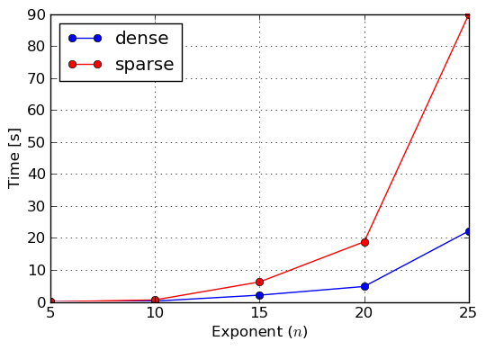
Benchmark: Exponentiation of 100% dense polynomial in x,y,z of total degree 3

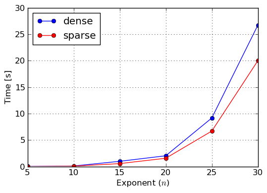
Benchmark: Exponentiation of 50% dense polynomial in x,y,z of total degree 3

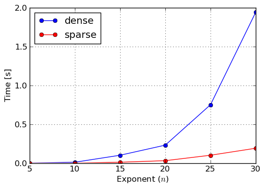
Benchmark: Exponentiation of sparse polynomial x + y + z

From those measures we can clearly see that sparse representation should be used as the main polynomial representation in near future, because it works better sparse and semi–dense inputs, thus covers most polynomials that can be encountered in real–life problems of symbolic mathematics. However, one should not go into a conclusion that dense representation is completely useless, because, as we already said, there are application in which dense polynomials can be found and thus SymPy and its users can still benefit from it.

Benchmarking ground types¶

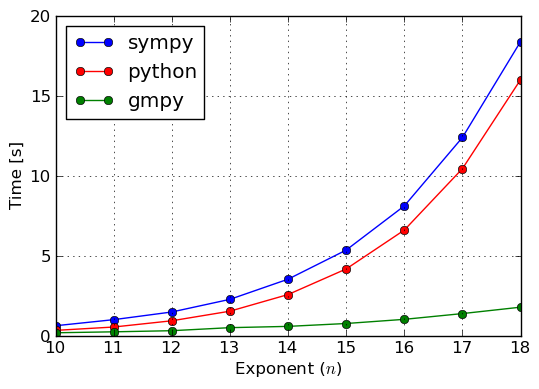
Enough was said about the theory of ground types, so lets now benchmark some examples and verify if this infrastructure gives any befits at all. We will solve two factorization problems over the integers: one with small coefficients (\pm 1) and the other with large coefficients (at most 56 digits). Results of this benchmark were collected in plots of figures Benchmark: Factorization of (small coefficients) and Benchmark: Factorization of (large coefficients).

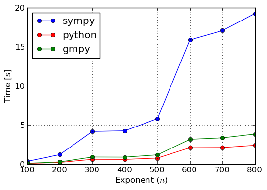
Benchmark: Factorization of x^n - 1 (small coefficients)

Benchmark: Factorization of (1234 x + 123 y + 12 z + 1)^n (large coefficients)

In the case of both benchmarks we see that computations with coefficients based on SymPy‘s Integer type are the slowest. This is because, Integer is a wrapper if Python’s int type and, thus, it adds significant overhead. From Benchmark: Factorization of (small coefficients) we see that int is a little better for small coefficients than gmpy’s mpz type. A reason for this might be that attribute access for the built–in type is highly optimized, whereas mpz has to use more general ways to access attributes. We did not investigate this, so there might be other explanations for this behaviour. However, for large coefficients mpz is unbeatable, because it implements asymptotically faster algorithms for integer arithmetics than int has.

In SymPy we use by default gmpy’s ground type, if the library is available on the system. When this is not the case, SymPy switches to Python’s ground types. SymPy‘s ground types are used usually for benchmarks, although, in the case of obsolete Python 2.4 and 2.5, which are still supported by SymPy, there is a need to use SymPy‘s Rational type to implement rational number domain, because Fraction type was introduced in Python 2.6.

Pure mode Cython in SymPy¶

To reduce the overhead of using pure mode Cython in SymPy to minimum, @cythonized decorator was introduced, which wraps original Cython’s decorators and adjusts them to SymPy’s needs. This is useful because we don not take advantage of many advanced Cython’s features. The only feature we need is to mark variables as native, because all native variables in SymPy, at least at this point, are integers, so there is not need to make things unnecessarily complicated. The decorator also allows to run SymPy in interpreted mode without Cython installation on the system. To achieve this, which is one of fundamental SymPy’s goals, we simply try import Cython and when this is not possible, we simply define an empty decorator.

Suppose we implement a function for rising a value to the n–th power, power() in this case. For this task we employ classical repeated squaring algorithm. A sample implementation goes as follows:

@cythonized('value,result,n,m')
def power(value, n):
    """Raise ``value`` to the ``n``--th power. """
    if not n:
        return 1
    elif n == 1:
        return value
    elif n < 0:
        raise ValueError("negative exponents are not supported")

    result = 1

    while True:
        n, m = n//2, n

        if m & 1:
            result *= value

            if not n:
                break

        value **= 2

    return result

The function can be run in both interpreted and compiled modes. To tell Cython that power() is ready for compilation, we use @cythonized decorator, in which we declare four variables as native: value, result, n and m. All four will have int type assigned during translation to C code. Two of those variables are input to the function. Cython is enough clever to automatically convert Python integers to native integers if necessary. The same can happen the other way in return statement. It is important to note that in interpreted mode Python uses arbitrary length integers, so we can compute arbitrary powers using power() function. This situation changes in compiled mode because we are restricted by machine types — we can store at most 32–bit or 64–bit values in native variables, depending on the actual architecture for which this piece of code was compiled. Such difference can have serious consequences, like wrong results of computation, if pure mode Cython was used without understanding of the behavior of this code on different platforms. This shows that developers have to be very careful about which variables should and which should not be marked as native. The general advice is to use native variables for loop indexes and auxiliary storage which we can guarantee to remain in right bounds. There are, however, cases where native variables can be used for doing actual computations, because it might be unrealistic to use larger values that 32–bit long. A good example is divisors(), which computes all divisors of an integer.

In polynomials manipulation mode we marked all loop index variables and some auxiliary variables on the lowest level as native. At this moment no coefficient arithmetics is done natively. It would be, however, very convenient in future to take advantage of native coefficient arithmetics when computing with polynomials over finite fields. In most practical cases in SymPy, coefficients which arise over finite fields are half–words, so arithmetics (especially including multiplication) can be done in a single machine word (32 bits). We could also consider allowing 64–bit words, if architecture supports this, to widen the range of application of optimized routines.

To take advantage of Cython in SymPy, the user has to compile it. By default SymPy ships only with bytecode modules and scripts for compiling them, if Cython is installed on the system. Assuming that GNU make is installed, then compiling SymPy is as simple as typing make at a shell prompt in the main directory of SymPy source distribution. If GNU make is not available, then the user has to issue the following command:

python build.py build_ext --inplace

from the same directory. This command tells Cython to compile all modules in SymPy, which have functions or methods marked with @cythonized decorator. The compilation is done in–place, meaning that there will two additional files for each Python source file: *.pyc file with bytecode and a compiled dynamically linked library. If --inplace was omitted, then Cython would store compiled modules in a separate directory, which would make running SymPy with compiled modules complicated.

Benchmarking pure mode Cython¶

It is very cheap to employ pure mode Cython in Python code. Does it, however, bring any improvement over pure Python? First experiments with pure mode Cython, which we conducted in SymPy, showed that the befit can be substantial or even impressive, giving over 20 times speedup for particular small functions, in which we could use native variables for coefficient arithmetics. The main subject of those experiments was divisors`() function. Those experiments were, however, artificial and for real–life cases speedup is not that big, but still worthy consideration, especially we take the tiny cost of pure mode Cython (one additional line per function or method).

Suppose we expand a non–trivial expression ((x + y + z)^{15} + 1) \cdot ((x + y + z)^{15} + 2) and then we want to factor the result back. We are interested only in factorization time. We perform the same computation in pure Python and pure mode Cython:

• pure Python

  >>> f = expand(((x+y+z)**15+1)*((x+y+z)**15+2))
  
  >>> %time a = factor(f)
  CPU times: user 109.45 s, sys: 0.01 s, total: 109.47 s
  Wall time: 110.83 s
  
  >>> %time a = factor(f)
  CPU times: user 109.31 s, sys: 0.03 s, total: 109.34 s
  Wall time: 110.68 s
  

• pure mode Cython

  >>> f = expand(((x+y+z)**15+1)*((x+y+z)**15+2))
  
  >>> %time a = factor(f)
  CPU times: user 72.09 s, sys: 1.02 s, total: 73.11 s
  Wall time: 74.18 s
  
  >>> %time a = factor(f)
  CPU times: user 72.81 s, sys: 0.04 s, total: 72.85 s
  Wall time: 73.74 s
  

We can see that for this very particular benchmark we obtained 1.5 times speedup. This is not 20 times, but still can be considered important, especially when such long computation times are involved. More throughout timings can be found in figures Benchmark: Exponentiation of and Benchmark: Factorization of over integers, where we exponentiated and factored polynomials for various exponents and degrees, respectively.

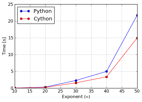
Benchmark: Exponentiation of (27 x + y^2 - 15 z)^n

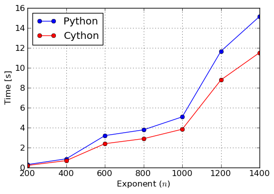
Benchmark: Factorization of x^n - 1 over integers

In future we expect even better improvements when native variables will be used for coefficient arithmetics. Every algorithm which uses modular approach, which include algorithms for factoring polynomials, computing GCD or resultants, will benefit from this, because coefficients arising on the intermediate steps in those algorithms are usually half–words (computations are done in small finite fields). How to achieve this, without compromising functionality and correctness, is a subject for future discussion.